Finding the Tree of Life in Evo 2
Evo2 was trained only to predict the next letter of DNA. Read its activations back and the bacteria it has seen are arranged the way evolution arranged them — once the distance is measured the right way.
| Building | A faithful replication that reads bacterial phylogeny out of a genomic model's embeddings |
| Models | Evo2-7B (blocks.24) · tetranucleotide baseline · label-shuffle control |
| Topics | Life sciences · Neural geometry · Evaluation & benchmarking |
Every genome carries a record of its ancestry. Two species that split from a common ancestor long ago have drifted far apart in sequence; two that diverged recently still read almost alike. Biologists spend careers turning that signal into the tree of life, the branching map of who descends from whom. A genomic foundation model like Evo2 is trained on raw genomes for one narrow task, predicting the next nucleotide, and is never shown a species label or a tree. The question this recipe takes up, following Goodfire's phylogeny-manifold study, is whether that tree is nonetheless sitting inside the model, recoverable from its activations.
Silico can take this published method and turn it into a runnable plan, executing the whole pipeline as a single experiment: from the steps alone, one dispatched run selects the 2,395 species, harvests Evo2's layer-24 embeddings for each genome, measures distances against the GTDB reference tree, and computes the baselines and controls alongside. The findings come back reproduced inside that one run: embedding distance tracks evolutionary distance at ρ 0.74, a graph geodesic at r 0.81, far above a sequence-composition baseline (0.31) and a label-shuffle control (0.02).
Key takeaways
- A published method becomes a runnable experiment. Silico turns a protocol like Goodfire's phylogeny-manifold steps into an editable plan and dispatches it, so reproducing a biological-model result is a scoping conversation rather than a from-scratch build.
- Model internals are harvested and probed end to end. A single run pulls Evo2's layer-24 embeddings across 2,395 genomes, lays out the manifold, and scores it against ground truth (the GTDB tree), with the activation access and cluster compute handled by the workflow.
- Findings arrive already pressure-tested. The composition baseline and the label-shuffle control are computed in the same run, so a claim that the model has internalized phylogeny comes with the confounds it has to beat.
Recreate the manifold
The scoping prompt was concrete: recreate Goodfire's tree-of-life manifold for Evo2, with four points of the protocol that the post leaves implicit spelled out — how species are sampled, how genome windows are filtered, how species pairs are sampled for the correlation, and how the geodesic is built. Before any compute was dispatched, an exploration of the workspace found a complete prior pipeline already there: a working Evo2 environment, the GTDB reference tree, the OpenGenome2 genomes, and cached model weights. The task turned from a build into a careful correction.
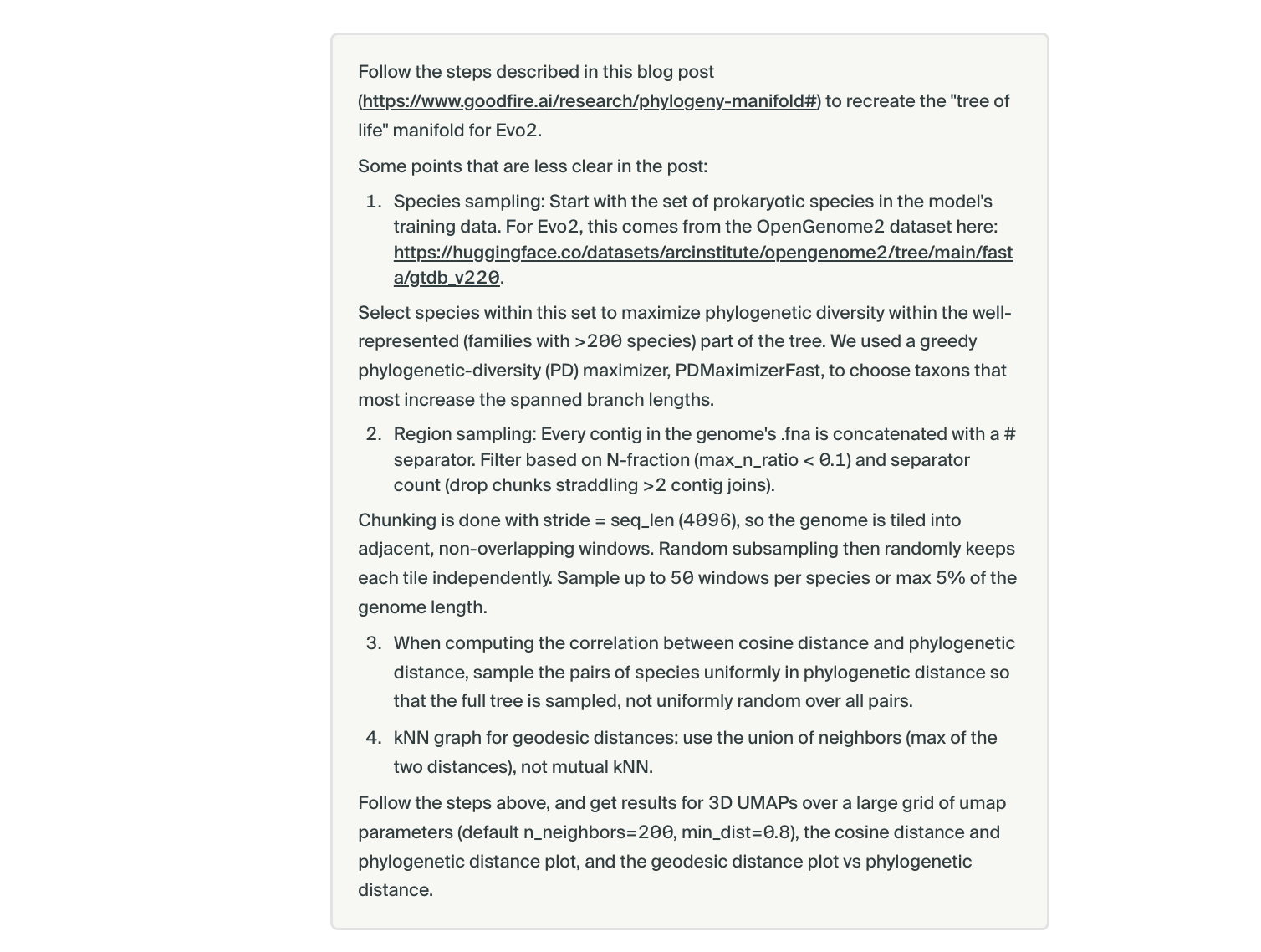
The plan stayed a living draft once it was running. Partway through the harvest, a question surfaced about the species filter: the rule to keep only well-represented families (more than 200 species) was counting family sizes across all of GTDB, when it should count only the species actually in the model's training distribution. The run was interrupted, the selection redone on the in-distribution counts, and the harvest restarted before compute was spent on the wrong set. Correcting the design mid-flight is the kind of steering the workflow is built for.
Does distance in the model track evolution?
For each of the 2,395 species, the run tiled its genome, embedded each window through Evo2-7B at layer 24 (the residual stream out of block 24), pooled the activations into one vector per species, and measured angular distance between species in that space. The ground truth is patristic distance on the GTDB tree: the total branch length walked from one species to another, short for recent cousins, long for lineages that parted in the deep past.
The explorer at the top of this page is that space: the model's embeddings flattened to three dimensions beside the real GTDB tree for the same species. Color by a taxonomic rank and the groups the model invented, with no biology supervision, fall into the same arrangement as the tree it was never shown. A flattened picture can invent structure that is not really there, so it is a companion to the measurement, not the proof. The proof is in the distances. On pairs sampled uniformly across evolutionary distance, angular distance in the model tracks patristic distance at Spearman ρ = 0.74. Tracing the shortest path between two species when each step may only hop to a near neighbor, a graph geodesic, lines up best of all, at Pearson r = 0.81 on the k-nearest-neighbor graph that first becomes fully connected at k = 17.
The decisive choice is the sampling. Averaged over all species pairs, the same embeddings give only ρ 0.32, because distant pairs dominate the tree and compress into a narrow, saturated band of angles where no trend is left to find. Sampling evenly across the distance range gives close relatives a fair say, and the trend reappears. That choice is the honest way to ask the question, and stating it plainly is part of the result.
Rule out the boring explanations
A correlation this clean invites the skeptical question: is the model really reading evolution, or is the number an artifact of the embeddings or the pipeline? The run answered with two references computed on the same pairs, and the gap between them is what makes the result convincing.
Two more checks keep the result honest. Changing how each genome window is pooled barely moves it, so it does not hang on one arbitrary choice. Centering the embeddings first actually lowered the correlation, to 0.66, so the raw embeddings were kept as the primary readout and the comparison reported rather than hidden.
When to reach for this
A model trained on a narrow prediction task can absorb deep structure about the world as a side effect. Whenever there is reason to suspect that, the same recipe applies: pick the structure that might be hiding in the model and read it straight out of the activations. The loop transfers directly:
- Name the structure you suspect is there. State the quantity the model might have internalized concretely enough to measure, the way phylogeny became angular distance between species here.
- Find a trustworthy ground truth. The readout is only as honest as what it is checked against; here it was the GTDB tree, but it can be any reference that is independent of the model.
- Measure on the right sample. When the comparison set is skewed, sample across the variable of interest before believing a null or a weak result. All-pairs averaging hid this signal until the pairs were balanced across evolutionary distance.
- Compute the controls in the same run. A composition baseline and a label-shuffle control are what turn "the embeddings know X" into a defensible claim.